In power markets, every forecast carries uncertainty. Transmission lines trip without warning, weather patterns shift, and load and renewable output diverge from expectation for any number of physical and behavioral reasons. In a prior post we discussed how probabilistic inputs can help us reason about that uncertainty directly. Here, we look at the methodology underneath: how we reconstruct historical system states well enough to train, validate, and stress-test the models that produce those forecasts.
Point-in-time vs Perfect Information Differentiation
When forecasting with physics-based models, we distinguish between the physical model itself (e.g., DCOPF) and the input data that drives it. Two questions arise: "Can my physical model capture real-world behavior?" and "Is my input data sufficiently accurate?" We answer them with two flavors of backtest. A perfect information backtest uses all data we have today, including actual loads, submitted offers, and other information that was not available during the test period. Because the inputs are clean, any gap between modeled and actual prices is attributable to the model itself; running with actuals also lets us reconstruct unobserved grid states like line flows, historical congestion drivers, and binding operational constraints. This creates a physically consistent foundation for the probabilistic models built on top.
A point-in-time backtest uses only the information that would have been available during the test period and measures how a deployed forecasting system would have performed. In energy markets, this distinction matters. Tests that accidentally incorporate the latest solar or wind conditions, meter-level demand data, or updated generation attributes can appear highly accurate in evaluation but fail in live operation due to these data leaks. Running both types of backtests lets us identify the source of forecast errors rather than just measure their combined effect. For example, the chart below shows solar generation data for one power plant in ERCOT. ERCOT publishes output data for power plants but at a 60-day delay, so that data is available for a perfect information backtest but not for a point-in-time test of any recent forecast.
The Distill Method
So far we've described the physical model as a well-defined fixed object where the input data are the only things that vary. This is only partially true. The physics of the system are well-defined, but market rules can be incorporated in slightly different ways and assumptions are often needed to blend information from different data sources. For example: How is real-time data merged with day-ahead data? How are cost curves approximated? How are loads downscaled? What ramp rates are used? What security constraints are considered? How are reserves modeled?
Distill provides reasonable defaults, but doesn't try to hide these nuances. Our modeling tools are designed to be approachable, flexible, and fast, giving you the ability to modify the underlying assumptions, run your own backtests, and tailor the results to your specific use case. Rather than creating a single forecast, we provide a modular framework and supporting data. Our cloud environment lets you run backtests and forecasts quickly, iterating on configurations and optimizing against whichever metrics matter most to your work.
High Level Assessment of a Backtest
Internally we've performed many backtests as we continually refine our model and default settings. Below we review results from one backtest that was performed during this calibration process. Here we're targeting ERCOT settlement point prices.
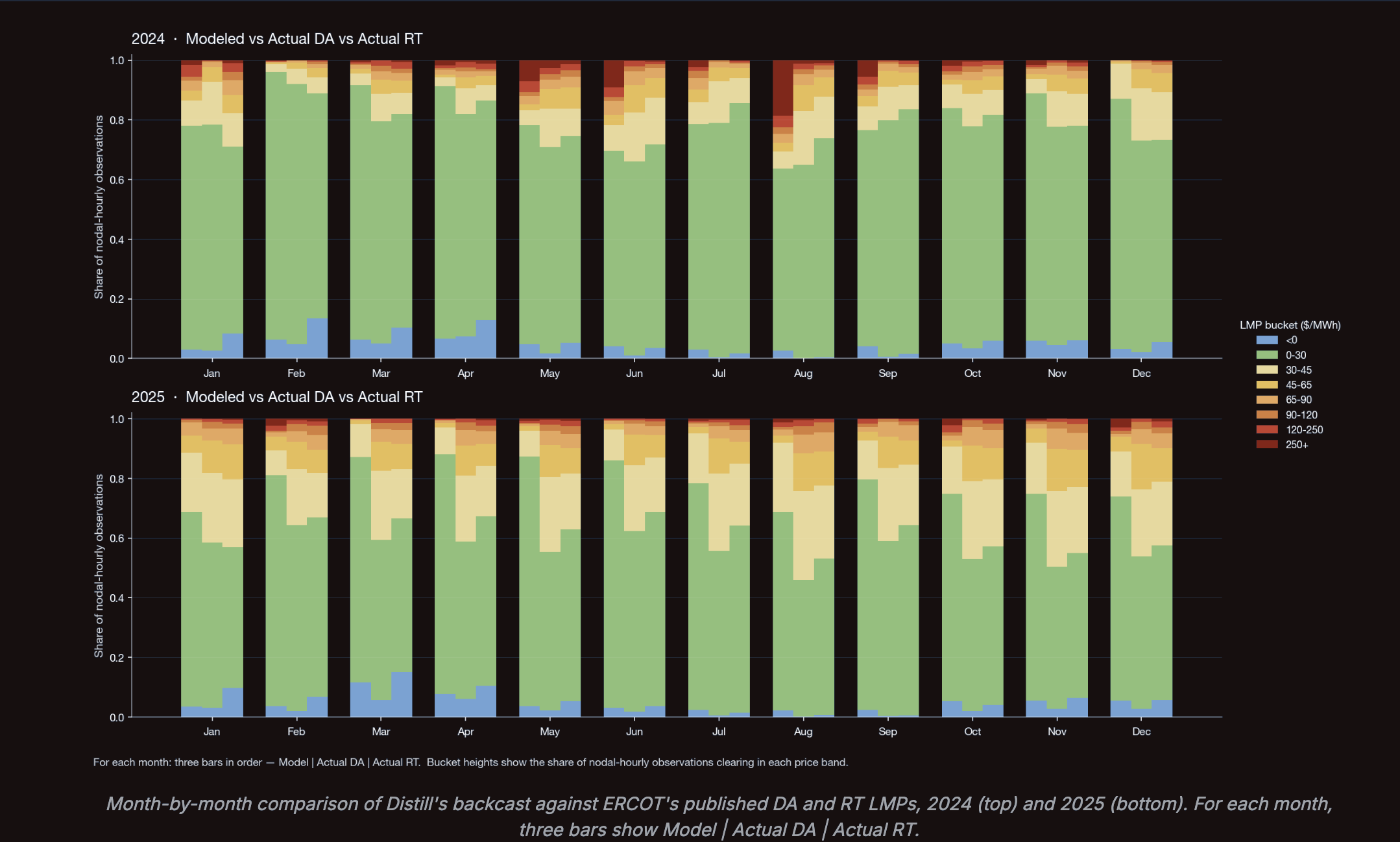
The results show that the model is capturing the bulk of the LMP distribution, but also reveals a few places where the model is still mis-calibrated. In August 2024 it overstates the scarcity tail, and in 2025 it under-prices the typical day by about $6. This suggests that this particular iteration of the model may have too much generation on average. To refine the model, we can dig in to the results at finer granularity: we slice the same comparison by region and by hour of day to find where each bias concentrates and identify systematic or subtle issues in the current model components that need to be improved.
Spatial and Hourly Diagnostics
The grid is in constant flux: new resources come online, new transmission constraints emerge as system topology evolves, and operational maximums are met on a regular cadence. Each of these reshapes how prices form. Therefore, absolute price error alone can be difficult to compare across zones, seasons, or years with materially different volatility profiles. Absolute price errors may also not be the metric most relevant to your use case. Spread accuracy, congestion directionality, and relative improvement over baseline forecasts often provide clearer insight into practical model performance.
The interactive below lets you step through twenty-one sample days from the same backtest. For each day, the maps show nodal LMPs at the hour you select with Model and Actual DA on a shared color scale, and the chart underneath pairs the diurnal LMP shape with the hour-by-hour spatial correlation between modeled and actual nodal prices.
A few patterns emerge as you step through the days. On clean alignment days, such as 2024-02-28 or 2024-10-05, both maps show the West Texas low-price wind cluster and the broad warming through central and east Texas in the same places, and the spatial correlation climbs through the afternoon into the evening peak. On harder days, such as 2025-10-28, the model under-clears the absolute level by several dollars per megawatt-hour but still reproduces the geographic gradient, telling us the tuning work belongs in the level calibration, not in the spatial assembly. The picker is sorted by date so the variant change between 2024 (load109) and 2025 (emp_lv) is easy to spot.
What This Means
A backtest on its own is not a forecast. It's the audit trail behind every forecast you can create with Distill: a way to confirm that the data assembly reconstructs what actually happened, the solver returns coherent prices, and the structural biases that remain are visible and addressable. Our solutions include full decomposable results, making analyses like the aggregate distributions, the spatial alignment, and the hour-by-hour spatial correlation above easy to create and access.
In the next post in this series, we will turn to point-in-time backtesting, where the assembly is constrained to use only the information that would have been available at the time of forecast. That is where we learn whether the model would have helped a trader, a developer, or an asset owner make a different decision under uncertainty.
In the meantime, behind these graphics are hundreds of simulations, compiled to demonstrate the varying system dynamics that appear under different input scenarios. If you would like to dig into the full dataset behind these charts and the underlying input series for each model variant, reach out. We are happy to share granular result sets and walk through how Distill is applying them in our work today.