
Before Bid-Close
We recently deployed our new DAM solver for all customers. This new iteration of our work shows marked accuracy improvements over our previous model.
For this model release, we’re publishing our internal backtest results across multiple metrics, including accuracy, timing, dispatch, and congestion.
| Settlement point | MAE | MAPE | Bias |
|---|---|---|---|
| Hub | $5.46 | 17.4% | −$1.83 |
| Node | $7.44 | 23.3% | −$1.81 |
Throughout this post, we go into finer resolution and detail than these headline metrics.
All of the results are point-in-time results, a methodology we’ve discussed in a previous blog post. As a reminder, point-in-time forecasting uses only the data available at 06:00 CT, well before DAM bid-close.1 These backtest results represent what would be available day-of for Distill users.2 For example, the DAM 03-15 backtest used only information available before bid-close on 03-14.
Our backtest window includes March 2026 to date. The beginning of 2026 marked the start of RTC+B, which altered the protocols significantly. Our forecasting methods depend on a rolling window of disclosure data, and March was the first full month of RTC+B disclosure data available to us.
If you’re not convinced by our results, check back in sooner rather than later; we’re always improving our models.
Price Accuracy
The model is evaluated on the fundamental goal of price accuracy.3 While the simulation procedure also results in other quantities (like LODFs, post-contingency line flows, etc.), those are largely in service of accurate prices.
Therefore, our model’s price accuracy is critical. We explore it below.
Time Series
We evaluate our results across time. Below is one of the model’s best weeks.
The Panhandle can produce extreme behavior due to congestion. However, even with the volatility inherent in that region, our HB_PAN results are still strong.
Distill simulates the power market at a bus-level resolution, and we return prices for buses and price nodes. Nodes are more recognizable than buses, so we’ve chosen a few interesting price node time series below.
However, not all weeks the same. The model performed relatively poorly in another week.
This week’s error is driven by two evening ramps. We capture the congestion pattern, but our system lambda is too low because we mischaracterize the scarcity in ancillary services. Under RTC+B, energy and ancillaries co-optimize, and missing scarcity in one will drive up the other. For instance, on 07/22 HE22, we broadly miss ancillaries:
| ERCOT | Distill | |
|---|---|---|
| NSPIN | $62.66 | $16.18 |
| ECRS | $27.55 | $1.00 |
| RRS | $19.00 | $0.36 |
| RegUp | $22.04 | $0.94 |
The scarcity was likely driven by poor renewable generation that fell short of ERCOT’s forecast. Self-scheduled renewables enter into the solve by reducing net load. The poor forecast resulted in 2 to 7 GWs of unexpected demand (i.e. unexpected self-scheduled renewable shortfall) in the worst hours.
(We also ran a perfect information / hindcast backtest, which eliminates the forecasting error and purely evaluates the solver. On 07/21 and 07/22 with a perfect weather forecast, we observe a hub error of $0.92 and $1.18 respectively. Approximately 95% of the error on those days was due to a poor forecast rather than a bad powerflow model.)
However, even with a poor default renewables forecast, the model still does well and captures the market dynamics correctly.
Error Distributions
Below are distributions of hourly error for each hub and a handful of nodes. We use distributions to ensure that our model is well-calibrated and does not exhibit systematic overpricing or underpricing.
In general, we systematically underprice the error, as is evident in the bias. The mode of the distribution is above $0, so the bias is driven by a long left tail where we underprice scarcity (like in the time series above).
Duck Curve
ERCOT’s prices exhibit a classic duck curve shape. However, internally, we’ve observed that there are slight variations from season to season. Below are the duck curve plots for the hubs, but split by season:
- All: March to October
- Spring: March, April, May
- Summer: June, July, August
- Fall: September, October (to date)
Nodal Basis
Though Distill solves at a bus-level resolution, we’ll only show price nodes here. We’ve split the basis into on-peak and off-peak hours. For each node, the price is the mean of all hours in that window.
Model Timing
A secondary, but also important, metric on which we evaluate our model is timing. After all, accurate prices are useful only if they arrive in time for bid-close.
Currently, a single simulation (which includes hourly bus-level pricing) requires about 20 minutes. Our solver is parallelized and distributed in the cloud, meaning that it can run a large number of simulations at the same time. For instance, this 230-day backtest with 30 parallel workers took about 3 hours. A full year of hourly bus-level simulations would take about 4.5 hours.
Below, we show a group of 10 workers.
Speed increases are currently being trialed internally, and initial results show about 12 minutes per simulation (40% faster), meaning a full year of simulations would finish in 2.75 hours.
Furthermore, parallelism can be increased. While we were testing internally, we ran with fewer parallel workers than is optimal.
For probabilistic simulations within the same day, results are usually much faster due to some internal computation optimizations leveraged by Distill. As an example, 230 simulations of the same day with perturbed inputs would take much less time than 3 hours.
In an earlier blog post, we discuss the advantages of probabilistic forecasting, including the mitigation and exploration of risk from deterministic forecasts. However, this backtest was purely a deterministic forecast to evaluate the efficacy of our solver.
Generation, Ancillaries, and Congestion
Nodal prices are determined by the price of dispatch and congestion. It’s possible to forecast nodal prices as an independent entity, but we know that the prices are determined by the physical grid. Therefore, we also evaluate our model on the factors that directly produce these prices.
Here, we’ve aggregated the system-wide average dispatch per hour for four days, one from each week in the time series above.
Our error in wind and solar is largely driven by weather-forecasting errors. Those errors require altering dispatch from thermal units, which also drives their error up in turn. We use ERCOT’s wind and solar forecasts that are available before bid-close, but Distill’s product allows you to bring your own forecast and solve against that forecast. We believe that with more accurate proprietary forecasts, error would drop further.
Finally, because we solve at an hourly bus-level, we also solve constraints. The solver considers all of ERCOT’s monitored elements, and the model produces shadow prices and post-contingency line flows.
Because constraints drive prices for individual nodes, we measure our alignment with ERCOT. We assess constraint accuracy using a weighted F1 score, which accounts for false positives, false negatives, and the severity of the misses.
If we look at the congestion component for nodes affected by a given constraint for the hours where ERCOT binds that constraint, we find that nodal prices are more accurate than the F1 score would imply.
For instance, when we miss BRUNI, we find that the nodes affected by BRUNI generally track ERCOT. Below, we look at the most exposed4 node to BRUNI, which is CEDROHI_CHW1. We compare the congestion component of the price averaged for the hours that ERCOT bound that element.
After Bid-Close
We run backtests like these to benchmark our model’s accuracy. Before we started Distill, these are the types of backtests that we wished other commercial solutions would publish for traders.
We’re happy to share these results because we know that Distill will only get better over time. We’re continuously improving our models from insight generated internally at Distill and from customer feedback.
We’re also continuing to expand our product features, including a real-time model and a CRR model.
If you’re interested in learning more, setting up a demo, or wanting to sign on for a trial, reach out to us at info@distill.energy.
Appendix
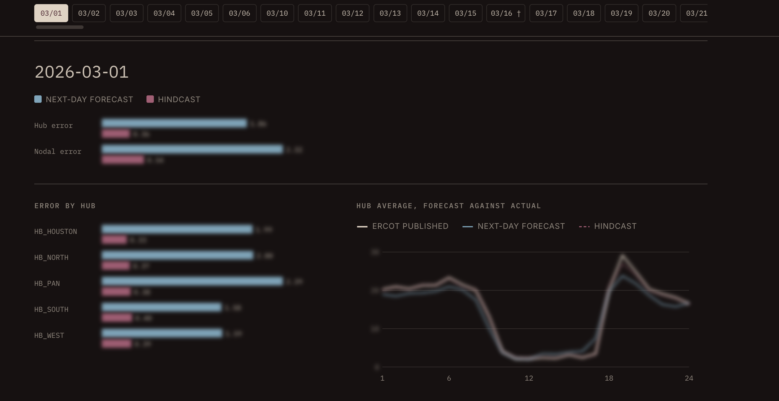
This blog contains high-level, demonstrative examples of our backtest results. A more comprehensive backtest is available: hourly hub error, constraint bindings, and awards for every day in the backtest. It can be found at Distill Labs.
Footnotes
1. We use only what is public by 06:00: the morning wind, solar and load forecasts, the reserve outlook, and the 60-day disclosures. ↩
2. For those who are interested, we also have results from perfect information backtests that analyzes solver physics and alignment with ERCOT. ↩
3. Price accuracy is not our only evaluation metric. Bus-level price is driven by congestion. If we analyze price accuracy solely at a hub level, extreme congestion misses - which could drive shadow to $1000 - would produce misses that are washed out by the aggregation at the hub. Therefore, we look at per-node price accuracy and congestion. ↩
4. We calculate the “most exposed” node by looking at the average shift factor of that node throughout the season in question. Shift factors do change over time, but our pricing comparison isn’t dependent on the averaged shift factor. We just use the shift factor to find the most interesting node for the analysis. ↩