Background
Financial markets are ubiquitous in Western society, but few are tightly coupled to complex physical systems, where the clearing mechanism itself is tied to the physics of the system. Deregulated wholesale electricity markets are a prime example. The price you see at a particular location is not just the outcome of supply and demand in the abstract — it is the outcome of supply and demand subject to the physics of the grid.
Most deregulated systems use multiple markets that work in concert to match electricity demand with generation while also providing reliable operation and incentivizing transmission improvements. Matching generation and demand within a single day is primarily accomplished by energy markets, which are the focus of this post.
Our goal is to introduce their basic form through the lens of optimal power flow (OPF) and use simple examples to highlight a few key features. Each example in this post is also paired with a live model in OPF Studio, one of Distill’s tools for building and solving DC optimal power flow problems. The links in each caption open the relevant example directly, so you can build intuition by modifying the example and exploring the impact of different parameters.
Economics of Generation and Demand
In a regional transmission system, there are generators that produce power and consumers like utilities, data centers, and industry that need power. These consumers are referred to as loads or collectively as demand. An energy market is a mechanism for connecting generators and loads. They are designed to dispatch the generation needed to meet a given load at minimum cost. If we ignore the transmission system entirely and pretend that all generation and all load sit at a single point (called a bus), then the least cost dispatch problem reduces to a typical supply curve: dispatch generators from cheapest to most expensive until total generation equals total demand. The cost of generators is dictated by the bid price they submit to the market. This is the merit order, and it is covered in more depth in Sonya's earlier post and the merit order explorer app.
Consider the simplest possible example: one bus, one load, and two generators — a cheap one and an expensive one. Suppose that both generators have 100 MW of capacity, but the cheap one offers to provide this power at $25/MWh, while the expensive one offers it at $60/MWh.
Now imagine two different situations, one where the load is 80MW and the other where the load is 150MW. In the first case, the cheap generator’s 100MW capacity is enough to cover the 80MW load and the market’s desire to find the least cost dispatch is obtained by fulfilling all 80MW of the load using the cheap generator. This is shown in the Figure 1.
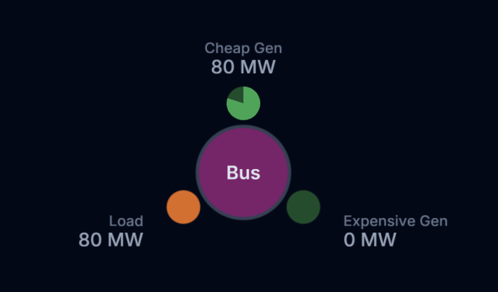
Figure 1: Single bus problem where the cheap generator’s 100MW of capacity is sufficient to fulfill the 80MW load. The green dots represent generators, and the orange dot represents the load. Click here to open the problem in OPF Studio.
In the second case, the load is increased to 150MW and the cheap generator is no longer sufficient to fulfill the load. Some combination of the cheap and expensive generation is needed. We could use 100MW of expensive generation and 50MW of inexpensive generation or even 75MW of each, but the option with the least cost is to use all of the cheap generation first and then use expensive generation. Minimizing the cost like this results in the solution shown in Figure 2.
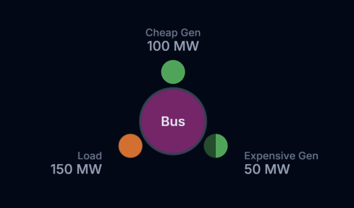
Figure 2: Single bus problem where a combination of cheap and expensive generation is needed to fulfill the load. Click here to open the problem in OPF Studio.
In the merit order, the last generator to be dispatched is called the marginal unit. This is the generator that would respond to an increase in load. Similarly, the cost of serving a unit increase in load is called the marginal price. In this example, the expensive generator is the only unit with capacity to fulfill load so it is the marginal unit and the marginal price is $60/MWh. This is also the clearing price in the market. Generation offered at prices below this are dispatched while generation offered at prices above this are not. In the first example, the marginal price was $25/MWh and came from the cheap generator.
Even though the cheap generator is willing to produce energy at $25/MWh in both cases, in the second case it is paid $60/MWh, the marginal price. The marginal price describes the value of power and all generators are paid that value. This example’s use of a single bus implies uniform pricing for all participants, but a generalized locational form of the marginal price arises when we consider transmission, this is discussed below.
Physics of Flow
We need sufficient generation to meet the demand, but we also need the ability to get energy from the generators to the load. In real systems, generators and loads are spatially distributed across multiple buses that are tied together with transmission lines, also referred to as branches. Buses are the connection points and branches are the connectors. Physics-based models of transmission are used to predict how power flows across branches and help operators control the power system.
There is a broad range of physics-based models with varying fidelities and computational expense. On one extreme is a model that simulates the full time-dependent 3D electric field around the transmission lines. This would be incredibly accurate but its computational expense and data requirements would prevent it from being practically useful. On the other extreme is a model that mostly ignores the physics and assumes we can move power across the system however we want. This would be fast to calculate, but wouldn’t sufficiently capture real system behavior. Useful models lie between these two extremes; they have sufficient fidelity but with reasonable computational expense.
Here we focus on the DC power flow (DCPF)1 class of models because they are the basis of many market mechanisms, including the day-ahead markets run by most ISOs. DCPF models capture enough physics to be useful to make day-ahead dispatch decisions while also being computationally feasible. Importantly, the structure of DCPF also enables locational marginal prices (LMPs) to be derived. These spatially variable market clearing prices are a key component of energy markets.
Combining Economics and Physics
Power flow models predict how power moves through the transmission system if generation and load were fixed. Energy markets on the other hand, are used to compute market prices (LMPs) and the corresponding generator dispatch (and storage, and flexible loads, but those are topics for another post). To accomplish this, we need to move beyond power flow into a class of problems called optimal power flow. The optimal in the name comes from the fact that we are optimizing for the least cost solution, just like in the market examples above.
Instead of a simple power flow model, optimal power flow represents a step towards a more comprehensive market model that incorporates
- a physics-based representation of flow
- the economics of generation
- safe physical limits of transmission components
- constraints that guarantee reliable operation
Market models extend the optimization approach from the "Economics of Generation and Demand" section by using a power flow model as a set of constraints in the optimization problem. In addition to minimizing generation costs while meeting demand, they also satisfy the physics and limitations of the transmission system. When the power flow model is DCPF, this combined optimization problem is called DC Optimal Power Flow, or DCOPF. It is what most system operators solve, in some elaborated form, to clear their day-ahead energy markets.
To see what changes once the transmission system enters the picture, consider a two-bus example. Imagine the cheap and expensive generators we used before, but spread across two buses with a single transmission line connecting them. Similar to generators, lines also have a capacity of how much energy they can transmit, which we call the line's "rating". Lines are said to be binding if the flow is at the rating.
First, consider the situation in Figure 3, where the line has a capacity of 100MW, which is enough capacity to carry all of the cheap generation. The solution is nearly identical to the single-bus case: the cheap generator dispatches to meet the load, the line carries that flow, and the marginal price at both buses is the cheap generator's offer price. The transmission system does not affect prices because the flow on the line is below its rating.
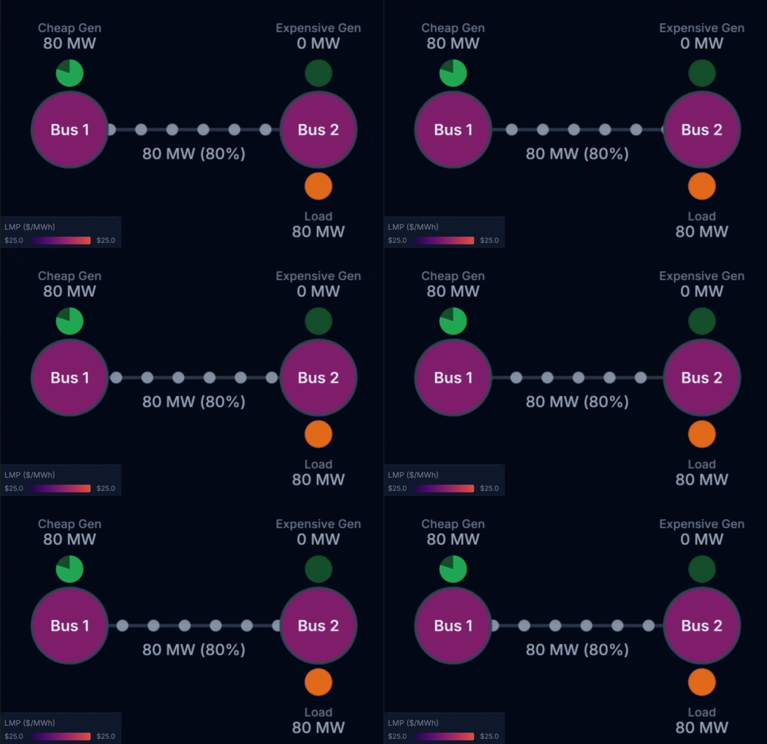
Figure 3: The line has sufficient capacity to carry the cheap power from Bus 1 to the load on Bus 2. The dispatch is identical to the case without any transmission line because the line rating of 100MW is sufficient to carry the power. Click here to open in OPF Studio.
Now imagine dropping the line rating to 50MW, which means only 50MW of cheap generation can be transferred from Bus 1 to Bus 2. The result is shown in Figure 4, with the key feature being the different prices on each bus. This spatial price difference results from congestion on the line.
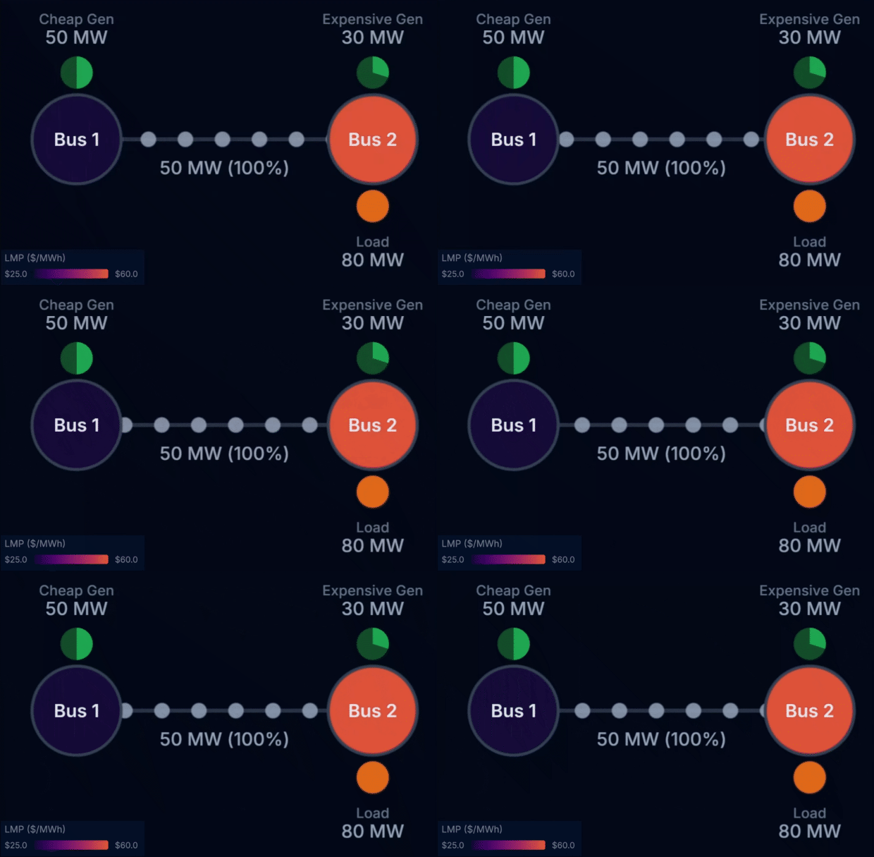
Figure 4: The line rating is dropped to 50MW and the line can no longer move enough power to fulfill the load with cheap generation. Both the cheap and expensive generators are below their limits, so both could respond to an increase in load on their respective buses. They are therefore the marginal unit on their bus. As a result, the LMP on each bus is the same as the generator’s offer price: $25/MWh on Bus 1 and $60/MWh on Bus 2. Click here to open this in OPF Studio.
LMPs generalize cleanly beyond the two-bus toy problem. In the DCOPF problem, every constraint has a shadow price — often called a dual price in the optimization literature — that indicates the marginal benefit of relaxing that constraint by one unit. The shadow price on a line flow constraint prescribes a value to transmission: it tells you how much the total system cost would decrease if that line could carry one more MW. In the Figure 4 example, the shadow price is $35/MW, which is precisely the difference in price between the cheap generator and the expensive generator. If one more MW was allowed to travel on the line, we could swap 1MW of expensive generation for cheap generation and the total cost would drop by their price difference: $35.
We are often focused on the shadow price associated with transmission constraints, but every other constraint has a shadow price too. Of particular importance is the power balance constraint that the power flow physics add to every bus: power flowing into each bus must match power flowing out. The shadow price on the power balance constraint is exactly the LMP.
Two-bus examples are useful for intuition, but real systems have thousands of buses, and congestion patterns can be subtle and counterintuitive where there are loops in the network. To get a feel for what this looks like at something closer to operational scale, OPF Studio ships with a calibrated zonal model of ERCOT — eight weather zones, a realistic generation mix, inter-zonal branches calibrated against the full nodal solve, and a 24-hour load profile derived from a real day-ahead-market case.
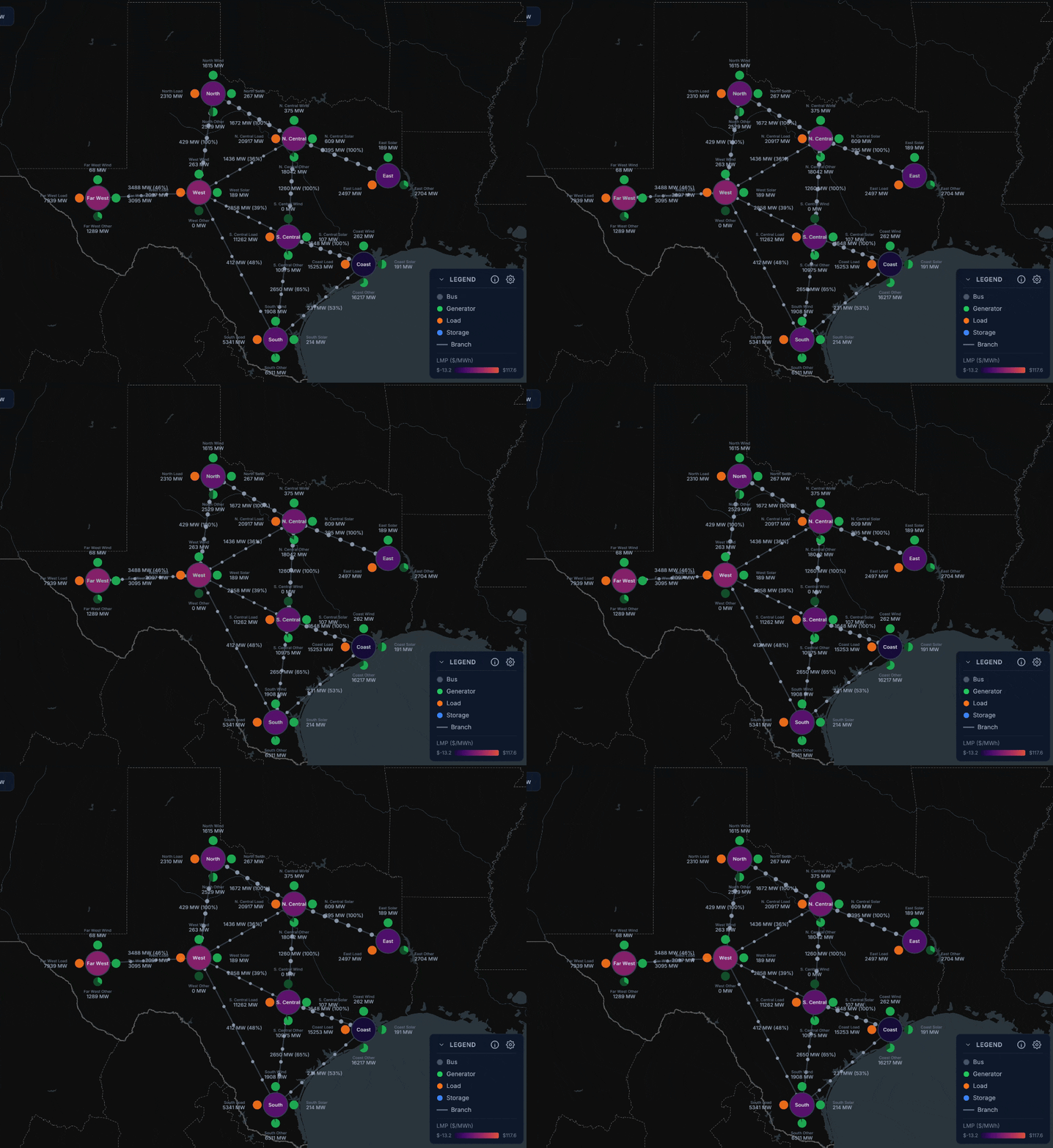
Figure 5: A zonal representation of ERCOT showing more complicated flows and dispatch. Click here to open in OPF Studio and explore in more detail.
Of note in the ERCOT example is how the LMPs and flows evolve over the day. Loads change hour by hour, wind output changes, and the marginal unit changes with them. Sometimes cheap West Texas wind sets the price, but other times a gas unit in Houston sets the price with a congested inter-zonal branch. The structure of the price map is a direct readout of where the binding constraints are at that hour.
Price Forecasting and Uncertainty
Running a market model built on DCOPF requires a lot of data — cost curves, load profiles, line ratings, generator capacities, ramp rates, and more. As discussed in Isaac's earlier blog post, we cannot always expect to know these values exactly; the inputs to the OPF problem are uncertain.
Probability is a natural mathematical language for describing uncertainty. We use probability distributions to model uncertainty in the OPF inputs (e.g., load, cost curves) and then propagate them through the OPF model to characterize uncertainty in the OPF outputs (e.g., prices, dispatch, line flows) with a probability distribution often called the predictive distribution. The complicated form of the OPF model results in predictive distributions that are not in a standard family (e.g., normal or uniform) and require the use of more complicated numerical techniques.
One way of characterizing the predictive distribution is by drawing random samples from the input distributions and then solving the OPF problem for each sample to obtain samples of the LMPs and other outputs. In practice we use more efficient sampling techniques, but the idea remains the same: generate a collection OPF solutions that represent the predictive distribution and can be used to statistically measure uncertainty and estimate risk. This general class of techniques is often referred to as Monte Carlo sampling and is particularly useful in the high dimensional problems we see in practice.
The shift from a single deterministic solution to an entire predictive distribution changes the form of the model output:
- Instead of one number for the LMP we now have a distribution over LMPs and can assess risk more accurately.
- Instead of one dispatch schedule, we have a family of schedules and can investigate the conditions that cause different generators to be used.
- Instead of one line flow, we have many possibilities and can compute the probability that a line is congested.
These are exactly the quantities a trader, a developer, or a planner cares about, but point forecasts hide them.
OPF Studio natively supports uncertainty quantification. Any input — load, generator capacity, marginal cost, branch parameters — can have a probability distribution attached to it. Figure 6 shows the impact of adding uncertainty to the load in the simple two-bus problem we used before. This example also adds a time component where the load varies from 30MW (below 50MW line limit) to 80MW (above 50MW line limit) throughout a 24 hour period.
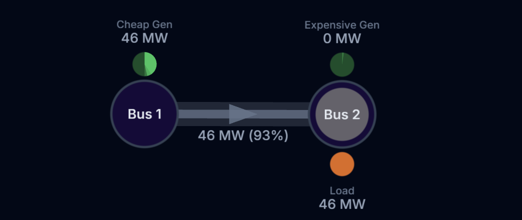
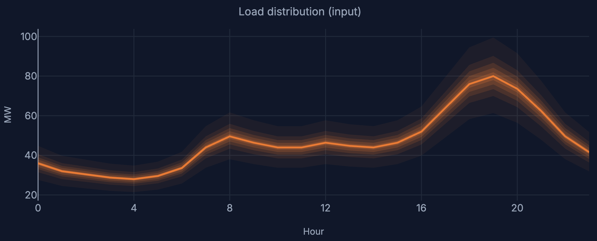
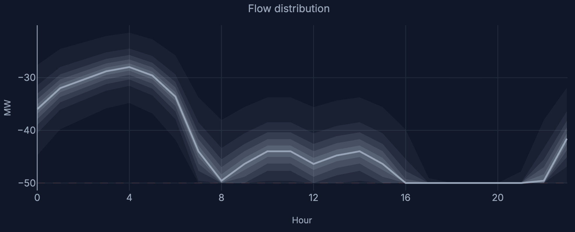
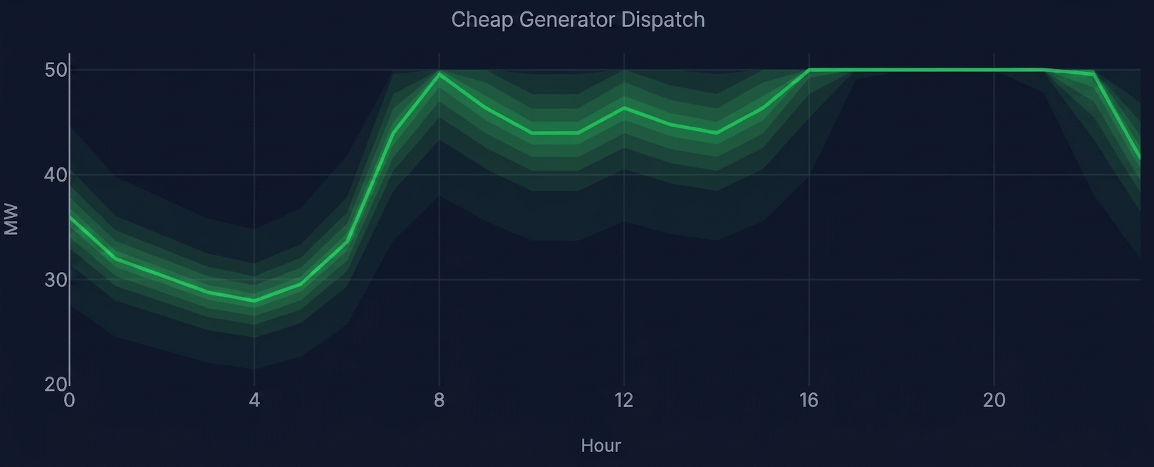
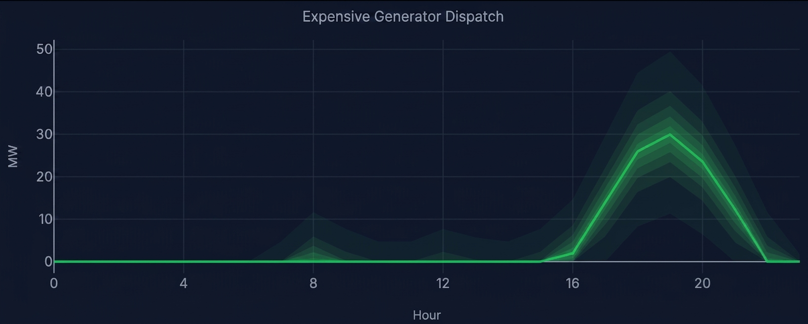
Figure 6: Results for the two bus problem with an uncertain time-varying load. The load is shown in orange and the result of propagating that to the line flow and generator dispatch (outputs of OPF) are shown in subsequent plots. The shaded regions in the plots show different quantile regions (e.g., region between 10%-90% quantiles) and thus represents the uncertainty in the quantity. Click here to open in OPF Studio.
Even this simple two bus problem shows interesting behavior when uncertainty is added. In hours 1-6, the load is below the transmission rating of 50MW. As a result, the cheap generator always matches the load and the load uncertainty is mapped completely into uncertainty in the cheap generator dispatch. There is no uncertainty in the expensive generator’s dispatch.
In hours 17-20 however, the load is almost always larger than the 50MW line limit. As a result, the cheap generator dispatch has no uncertainty during these hours; it’s fixed at the 50MW capacity of the line. All of the load uncertainty maps to the expensive generator.
This behavior demonstrates how difficult uncertainty quantification can be with OPF problems. It is not sufficient to simply add an error bar onto an existing OPF solve because the predictive distribution is highly variable, often skewed, and contains strong correlations. Characterizing these features is critical to accurately quantifying risk.
Wrapping Up
We've walked through a single-bus economic dispatch, the physics of how power actually flows on a network, the OPF problems underpinning energy markets, and finally through the impact of uncertainty on OPF results. Each step layered one more piece of realism onto the model. The result is a complex system with interesting dynamics, but one that is ultimately built on understandable concepts. At Distill, we are working to demystify the complexity of this system and enable anyone interacting with the grid to quantify its uncertainty and to manage their risk.
If you'd like to explore further, every example in this post is a live system in OPF Studio. Change the offers, tighten a line, add a wind farm, turn on uncertainty, and watch what happens to the prices.
Footnotes
1. DC power flow (DCPF) is not the same as “direct current” (DC) electricity. The "DC" in DCPF is a misnomer. The model still approximates alternating current (AC) flow through the transmission system. The DCPF equations are a linearization of the nonlinear AC power flow equations and the name comes from the fact that the equations look structurally like the equations for a DC resistive network — power flowing along a line is proportional to the angle difference across it, the way current in a DC circuit is proportional to the voltage difference. But in DCPF the physical system being modeled is still the flow of AC power through the grid. ↩